Tara Javidi

Consider exchangeable random variables ${X_1, \ldots, X_n, \ldots}$ . A couple of facts seem quite intuitive:

Statement 1. The “variability” of sample mean ${S_m = \frac{1}{m} \sum_{i=1}^{m} X_i}$ decreases with ${m}$ .

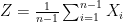
Statement 2. Let the average of functions ${f_1, f_2, \ldots, f_n}$ be defined as ${\overline{f} (x) := \frac{1}{n} \sum_{i=1}^{n} f_i(x)}$ . Then ${\max_{1\leq i \leq n} \overline{f}(X_i)}$ is less “variable” than ${\max_{1\leq i \leq n} f_i (X_i)}$ .

To make these statements precise, one faces the fundamental question of comparing two random variables ${W}$ and ${Z}$ (or more precisely comparing two distributions). One common way we think of ordering random variables is the notion of stochastic dominance:

$\displaystyle W \leq_{st} Z \Leftrightarrow F_W(t) \geq F_Z(t) \ \ \ \mbox{ for all real } t.$

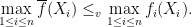
However, this notion really is only a suitable notion when one is concerned with the actual size of the random quantities of interest, while, in our scenario of interest, a more natural order would be that which compares the variability between two random variables (or more precisely, again, the two distributions). It turns out that a very useful notion, used in a variety of fields, is due to Ross (1983): Random variable ${W}$ is said to be stochastically less variable than random variable ${Z}$ (denoted by ${\leq_v}$ ) when every risk-averse decision maker will choose ${W}$ over ${Z}$ (given they have similar means). More precisely, for random variables ${W}$ and ${Z}$ with finite means

$\displaystyle W \leq_{v} Z \Leftrightarrow \mathbb{E}[f(X)] \leq \mathbb{E}[f(Y)] \ \ \mbox{ for increasing and convex function } f \in \mathcal{F}$

where ${\mathcal{F}}$ is the set of functions for which the above expectations exist.

One interesting, but perhaps not entirely obvious, fact is that this notion of ordering ${W\leq_v Z}$ is equivalent to saying that there is a sequence of mean preserving spreads that in the limit transforms the distribution of ${W}$ into the distribution of another random variable ${W'}$ with finite mean such that ${W'\leq_{st} Z}$ ! Also, using results by Hardy, Littlewood and Polya (1929), the stochastic variability order introduced above can be shown to be equivalent to Lorenz (1905) ordering used in economics to measure income equality.

Now with this, we are ready to formalize our previous statements. The first statement is actually due to Arnold and Villasenor (1986):

$\displaystyle \frac{1}{m} \sum_{i=1}^{m} X_i \leq_v \frac{1}{m-1} \sum_{i=1}^{m-1} X_i \ \ \ \ \ \ \ \ \ \ \ \ \mbox{for all }\ \ m \in \mathbb{N}.$

Note that when you apply this fact to a sequence of iid random variables with finite mean ${\mu}$ , it strengthens the strong law of large number in that it ensures that the almost sure convergence of the sample mean to the mean value ${\mu}$ occurs with monotonically decreasing variability (as the sample size grows).

The second statement comes up in proving certain optimality result in sharing parallel servers in fork-join queueing systems (J. 2008) and has a similar flavor:

$\displaystyle \max_{1\leq i \leq n} \overline{f}(X_i) \leq_v \max_{1\leq i \leq n} f_i (X_i).$

The cleanest way to prove both statements, to the best of my knowledge, is based on the following theorem first proved by Blackwell in 1953 (later strengthened to random elements in separable Banach spaces by Strassen in 1965, hence referred to by some as Strassen’s theorem):

Theorem 1 Let ${W}$ and ${Z}$ be two random variables with finite means. A necessary and sufficient condition for ${W \leq_v Z}$ is that there are two random variables ${\hat{W}}$ and ${\hat{Z}}$ with the same marginals as ${W}$ and ${Z}$ , respectively, such that ${\mathbb{E}[\hat{Z} |\hat{W}] \geq \hat{W}}$ almost surely.

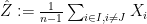
For instance, to prove the first statement we consider 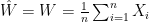${\hat{W} = W = \frac{1}{n} \sum_{i=1}^n X_i}$ and ${Z = \frac{1}{n-1} \sum_{i=1}^{n-1} X_i}$ . All that is necessary now is to note that ${\hat{Z} : = \frac{1}{n-1} \sum_{i\in I, i \neq J} X_i}$ , ${J}$ is an independent uniform rv on the set ${I := \{1,2, \ldots, n\}}$ , has the same distribution as random variable ${Z}$ . Furthermore,

$\displaystyle \mathbb{E} [ \hat{Z} | W ] = \mathbb{E} [ \frac{1}{n} \sum_{J=1}^{n} (\frac{1}{n-1} \sum_{i\in I, i \neq J} X_i ) | W ] = \mathbb{E} [ \frac{1}{n} \sum_{j=1}^{n} X_j | W ] = W.$

Similarly to prove the second statement, one can construct ${\hat{Z}}$ by selecting a random permutation of functions ${f_1, \ldots, f_n}$ .

Information Theory b-log

Author Archives: Tara Javidi

Comparing Variability of Random Variables