Shannon’s rate-distortion theory gives the optimal tradeoff between compression rate and fidelity, as measured by expected average distortion, if the distortion function is bounded. Here we show how to extend this for non-finite distortion metrics that strictly forbid certain reconstructions.
Distortion:
We will assume that the information source  has finite support, and the observed samples
  are i.i.d. with a known distribution
  . Let
. Let  be a distortion function used for measuring fidelity, where
  is the reconstruction. The average distortion for a sequence of source samples and reconstructions is the average of
  .
.
Rate Constraint:
The rate constraint imposed by rate-distortion theory allows  information symbols to be encoded as a block, where is specified by the designer of the encoding. The encoder maps the symbols to
  bits. A decoder then produces the best possible reconstruction, with respect to the distortion metric, based only on the bits of description.
Expected Distortion:
We say that  is achievable at rate
  if there exists a block-length and an encoder and a decoder operating with rate constraint such that the averaged distortion is less than in expected value. The average distortion is random because the information source is random and the encoder and decoder may achieve a different average distortion for different encodings, thus the need to consider the expected value.
Rate-distortion Function:
Let  be the infimum of rates such that is achievable at rate .
Rate-Distortion Theorem (expected distortion, known result):
For a source distribution , if is bounded,
where mutual information  is measured with respect to
  .
.
The above theorem is restricted to bounded distortion functions. Since has finite support and the optimal choice of Y also has finite support, an unbounded distortion function implies that the distortion is infinite for some pairs of values. That is, some pairs (x,y) are strictly forbidden, no matter how unlikely they are to occur. This cannon be guaranteed at the rates demanded by the rate-distortion theorem stated above.
Excess Distortion:
An alternative definition for achievability, known as excess distortion, requires that the average distortion be less than with high probability. That is, is achievable at rate if for any  there exists a block-length and an encoder and a decoder operating with rate constraint such that the averaged distortion is greater than with probability less than
  .
.
For bounded distortion functions, excess distortion is a stronger requirement than expected distortion. It’s insightful that the rate-distortion function doesn’t change even with this stronger requirement (see theorem below). However, for unbounded distortions, the excess distortion requirement allows an chance of “error.” Even if the distortion is infinite during those occurrences, the achievability criterion will still be met. So it cannot strictly forbid any reconstructions. This is why the following theorem does not require any condition on the distortion function.
Rate-Distortion Theorem (excess distortion, known result):
Under the excess distortion requirement, for a source distribution ,
Under the expected distortion requirement, one may wonder what the rate-distortion function is in general, for non-finite distortion measures. This curiosity is reflected in classic information theory texts from decades past and is the subject of this post. Csiszar’s and Korner’s 1981 textbook dances around this question, containing all the pieces but not connecting them together. I will make references to the second edition of their book.
Safe Value for :
The first idea one might consider is to identify cases where the rate-distortion function in the theorems above is still accurate. You might arrive at the following: If has a safe value of that always produces finite distortion for any  , then the encoder can add a single additional message. That message tells the decoder to produce the safe value of for the entire sequence. This message is only used when the encoder cannot find a valid reconstruction in the codebook with distortion less than infinity, which should be rare. One additional message does not change the asymptotic rate.
This observation is exercise 7.13 in Csiszar-Korner, which credits Gallager’s 1968 textbook. I will touch on Gallager’s bound momentarily.
Example of Conflict:
Before continuing, it will be beneficial to give a simple example where a non-finite distortion measure requires a rate higher than the rate-distortion function in the theorems above. We need look no further than a binary source. Let the distortion function be zero if  and infinity if
  . Under the excess distortion requirement, any finite distortion can be achieved with rate
  . In other words, near-lossless compression is necessary and sufficient to achieve finite average distortion with high probability. On the other hand, it is not sufficient to guarantee finite distortion with probability one. Under the expected distortion requirement, perfect lossless compression is required, and a rate
  is necessary.
Gallager’s Bound (1968 textbook, Theorem 9.6.2):
We must assume that for each in the support of there is a value of that yields finite distortion under . If not, then the average distortion will be infinite with high probability regardless of the encoder. Now suppose that there is a subset  such that for each in the support of there is a
  that yields finite distortion under . This is a generalization of the safe value of mentioned previously—instead it is a safe set in which you can always find a safe , though it will need to be specified by the encoder.
Theorem (Gallager):
Under the expected distortion requirement, for a source distribution ,
The theorem above is achieved by creating a reserve codebook that enumerates the sequences in the set . In the rare cases where the encoder cannot find a good reconstruction sequence in the primary codebook, it instead specifics a safe sequence from the reserve codebook.
Now the main point of this post.
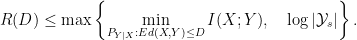
Non-Finite Rate-Distortion Theorem (average distortion, new result):
Under the expected distortion requirement, for a source distribution ,

Proof:
The above rate can be achieved by encoding separately for typical  sequences and atypical sequences. For the typical ones, design the encoder and decoder to assure an average distortion , and for the atypical ones just assure a finite distortion. The encoder can first specify the type to the decoder using negligible rate, so that the encoder knows which codebook to use. The maximization of the second term on the right-hand side accounts for each type being encoded separately. The rate of compression is determined by the highest rate.
Source coding is fundamentally different from channel coding in that there is a zero-error aspect of it that does not require any extra rate. We can efficiently obtain a perfect covering. If we consider error events to be instances where the average distortion exceeds , as in the excess distortion definition, then we can separate error events into two cases, those where is typical and those where it is not. The error probability when is typical can be made exactly zero using the same compression rate that achieves nearly zero error. The typical set is perfectly covered. So all of the error in source coding comes from being atypical. The proof that this occurs comes from the standard analysis using strong typicality. For an arbitrary typical , the probability of error is doubly-exponentially small, where the probability is with respect to a randomly generated codebook. The union bound over all typical sequences gives a doubly-exponential confidence that no typical will produce an error. Existence arguments complete the proof.
Since the scheme for achieving the theorem handles each type separately, there will be no errors (I’ve skipped over a uniform convergence bound that is needed to formalize this). Typical source sequences will yield distortion less than , and atypical sequences will yield finite distortion. The expected average distortion will meet the constraint.
One possible starting point to arrive at this result would have been to identify the rate required to guarantee finite distortion. This problem is combinatoric in nature—the distortion function only specifies which reconstructions are forbidden, and these constraints must be met with probability one. Because of this, the source distribution is no longer relevant. There are several equivalent formulas to express the minimum rate needed. A simple one can be obtained from Theorem 9.2 in Csiszar-Korner:

Then the formula for in the theorem can be understood in the following way: Encode for distortion , and when the encoder fails, use a reserve codebook that guarantees finite distortion. This sounds similar to Gallager’s method. The difference is that Gallager only gave a loose upper bound on the rate of the reserve codebook.
The converse to this theorem is immediate. Each of the two terms in the maximization corresponds to a necessary achievability requirement—average distortion and finite distortion with probability one. 
 -entropy (
 -entropy), Sharma-Mittal entropy,
 mutual information, Rényi mutual information, Tsallis mutual information, copula-based kernel dependency, multivariate version of Hoeffding’s
  and
and  , complex mutual information, Cauchy-Schwartz quadratic mutual information, Euclidean distance based quadratic mutual information, distance covariance, distance correlation, approximate correntropy independence measure,
  mutual information (Hilbert-Schmidt norm of the normalized cross-covariance operator, squared-loss mutual information, mean square contingency),
 (Spearman’s rank correlation coefficient, grade correlation coefficient), correntropy, centered correntropy, correntropy coefficient, correntropy induced metric, centered correntropy induced metric, multivariate extension of Blomqvist’s
  (medial correlation coefficient), multivariate conditional version of Spearman’s